Numerical Integration - Simpson's Rule

In numerical analysis, numerical integration constitutes a broad family of algorithms for calculating the numerical value of a definite integral, and by extension, the term is also sometimes used to describe the numerical solution of differential equations. The term numerical quadrature (often abbreviated to quadrature) is more or less a synonym for numerical integration, especially as applied to one-dimensional integrals.

The basic problem in numerical integration is to compute an approximate solution to a definite integral

 

to a given degree of accuracy. If f(x) is a smooth function integrated over a small number of dimensions, and the domain of integration is bounded, there are many methods for approximating the integral to the desired precision.

An important part of the analysis of any numerical integration method is to study the behavior of the approximation error as a function of the number of integrand evaluations. A method that yields a small error for a small number of evaluations is usually considered superior. Reducing the number of evaluations of the integrand reduces the number of arithmetic operations involved, and therefore reduces the total round-off error. Also, each evaluation takes time, and the integrand may be arbitrarily complicated. 

A 'brute force' kind of numerical integration can be done, if the integrand is reasonably well-behaved, by evaluating the integrand with very small increments. 

A large class of quadrature rules can be derived by constructing interpolating functions that are easy to integrate. 

Typically these interpolating functions are polynomials.

The simplest method of this type is to let the interpolating function be a constant function (a polynomial of degree zero) that passes through the point ((a+b)/2, f((a+b)/2)). This is called the midpoint rule or rectangle rule.

 

 

The interpolating function may be an affine function (a polynomial of degree 1) that passes through the points (a, f(a)) and (b, f(b)). This is called the trapezoidal rule.

 

For either one of these rules, we can make a more accurate approximation by breaking up the interval [a, b] into some number n of subintervals, computing an approximation for each subinterval, then adding up all the results. This is called a composite rule, extended rule, or iterated rule. For example, the composite trapezoidal rule can be stated as

where the subintervals have the form [k h, (k+1) h], with h = (b−a)/n and k = 0, 1, 2, ..., n−1.

Interpolation with polynomials evaluated at equally spaced points in [a, b] yields the Newton–Cotes formulas, of which the rectangle rule and the trapezoidal rule are examples. Simpson's rule is a Newton-Cotes formula for approximating the integral of a function  using quadratic polynomials (i.e., parabolic arcs instead of the straight line segments used in the trapezoidal rule).

Quadrature rules with equally spaced points have the very convenient property of nesting. The corresponding rule with each interval subdivided includes all the current points, so those integrand values can be re-used.
 

 

 

In sport and exercise biomechanics the data are most commonly available for wich the process of integration is appropiate are data from force platforms and accelerometers. The force data from force plataforms can be used to compute acceleration following Newton's second law (F = m * a). In this example, the process of integration enables the velocity to be obtained, and the process can be repeated in this velocity data in order to obtain displacement. This method can be applied in other type of biomechanics data, for example in EMG, like contractile impulse of activation. Integration of this type of data is best done using numerical integration.

The numerical integration method most commonly found in the literature in the area of ​​biomechanics is the Trapezoidal. However, studies such as Won (2000) shows that we must have concern for the error produced by the choice of the integration method to be used and the method of Simpson is the one with the lowest error. 

Simpson's rule can be derived by integrating a third-order Lagrange interpolating polynomial fit to the function at three equally spaced points. In particular, let the function  be tabulated at points , , and  equally spaced by distance , and denote . Then Simpson's rule states that

Since it uses quadratic polynomials to approximate functions, Simpson's rule actually gives exact results when approximating integrals of polynomials up to cubic degree. For example, consider  (black curve) on the interval , so that , , and .

Then Simpson's rule (which corresponds to the area under the blue curve obtained from the third-order interpolating polynomial) gives

 

whereas the trapezoidal rule (area under the red curve) gives  and the actual answer is 1. In exact form,

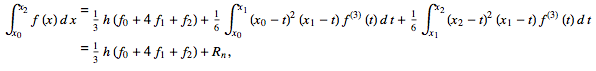
where the remainder term can be written as

 

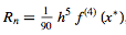
with  being some value of  in the interval .

An extended version of the rule can be written for  tabulated at , , ...,  as

where the remainder term is 

for some . 

Here's a link to download Matlab Code with a sub-program implemented in environment Matlab© to get the integration value of your signal with Simpson's Rule.
To use the function provided just save the file "simpson_gbiomech.m" in the same folder as the data to be analyzed. Then just call in your Matlab routine sub-program as follows in the example below:

Z=simpson_gbiomech(Y);      - computes an approximation of the integral of Y via the Simpson's method (with unit spacing). To compute the integral for spacing different from one, multiply Z by the spacing increment.

Z=simpson_gbiomech(X,Y);   - computes the integral of Y with respect to X using the Simpson's rule. X and Y must be vectors of the same length, or X must be a column vector and Y an array whose first non-singleton dimension is length(X). SIMPS operates along this dimension.


Note: you can specify the window which will be modified by inserting an index on the input variables.

References:

- Abramowitz, M. and Stegun, I. A. (Eds.). Handbook of Mathematical Functions with Formulas, Graphs, and Mathematical Tables, 9th printing. New York: Dover, p. 886, 1972.

- Davis, P. J.; Rabinowitz, P.. Methods of Numerical Integration. 

- Horwitz, A. "A Version of Simpson's Rule for Multiple Integrals." J. Comput. Appl. Math. 134, 1-11, 2001.

- Jeffreys, H. and Jeffreys, B. S. Methods of Mathematical Physics, 3rd ed. Cambridge, England: Cambridge University Press, p. 286, 1988.

- Stoer J.; Bulirsch R.. Introduction to Numerical Analysis. New York: Springer-Verlag, 1980. (See Chapter 3.)

- Trott, M. The Mathematica GuideBook for Programming. New York: Springer-Verlag, p. 105, 2004. http://www.mathematicaguidebooks.org/.

- Whittaker, E. T. and Robinson, G. "The Trapezoidal and Parabolic Rules." The Calculus of Observations: A Treatise on Numerical Mathematics, 4th ed. New York: Dover, pp. 156-158, 1967.

- Won, T. The comparison of among different numerical integration methods on the biomechanics of sport countermovement jump. 18º International Symposium on Biomechanics in Sports. Hong Kong, China: 2000. Available: <https://ojs.ub.uni-konstanz.de/cpa/article/view/2270/2123>

Big Hug!